Setup

Let’s start with using the R internal data cars:

data(cars)
x<-cars$speed # use the speed as predictor
y<-cars$dist # use the dist as response

Fit the models

Now, let’s get the polynomials for the variable x using the degree 3:

x1<-poly(x, 3, raw=TRUE)
x2<-poly(x, 3, raw=FALSE)
# check the resulted polynomials
head(x)

## [1] 4 4 7 7 8 9

head(x1)

##      1  2   3
## [1,] 4 16  64
## [2,] 4 16  64
## [3,] 7 49 343
## [4,] 7 49 343
## [5,] 8 64 512
## [6,] 9 81 729

head(x2)

##               1          2           3
## [1,] -0.3079956 0.41625480 -0.35962151
## [2,] -0.3079956 0.41625480 -0.35962151
## [3,] -0.2269442 0.16583013  0.05253037
## [4,] -0.2269442 0.16583013  0.05253037
## [5,] -0.1999270 0.09974267  0.11603440
## [6,] -0.1729098 0.04234892  0.15002916

poly() returns a matrix, with the first column corresponds to original data x, second column to the quadratic term x^2, third column to the cubic term x^3, etc.

As you see, there are two ways to generate polynomial data for a variable using poly() in R, depending on the option raw is TRUE or FALSE. When it is TRUE, the polynomials are simply x to the power of respective degrees. When it is FALSE, the polynomials are further normalized to be orthogonal among each other. We will see how different these two ways are in model fitting below.

m1<-lm(y ~ x1)
m2<-lm(y ~ x2)
# summarize the models
summary(m1)

## 
## Call:
## lm(formula = y ~ x1)
## 
## Residuals:
##     Min      1Q  Median      3Q     Max 
## -26.670  -9.601  -2.231   7.075  44.691 
## 
## Coefficients:
##              Estimate Std. Error t value Pr(>|t|)
## (Intercept) -19.50505   28.40530  -0.687    0.496
## x11           6.80111    6.80113   1.000    0.323
## x12          -0.34966    0.49988  -0.699    0.488
## x13           0.01025    0.01130   0.907    0.369
## 
## Residual standard error: 15.2 on 46 degrees of freedom
## Multiple R-squared:  0.6732, Adjusted R-squared:  0.6519 
## F-statistic: 31.58 on 3 and 46 DF,  p-value: 3.074e-11

summary(m2)

## 
## Call:
## lm(formula = y ~ x2)
## 
## Residuals:
##     Min      1Q  Median      3Q     Max 
## -26.670  -9.601  -2.231   7.075  44.691 
## 
## Coefficients:
##             Estimate Std. Error t value Pr(>|t|)    
## (Intercept)    42.98       2.15  19.988  < 2e-16 ***
## x21           145.55      15.21   9.573  1.6e-12 ***
## x22            23.00      15.21   1.512    0.137    
## x23            13.80      15.21   0.907    0.369    
## ---
## Signif. codes:  0 '***' 0.001 '**' 0.01 '*' 0.05 '.' 0.1 ' ' 1
## 
## Residual standard error: 15.2 on 46 degrees of freedom
## Multiple R-squared:  0.6732, Adjusted R-squared:  0.6519 
## F-statistic: 31.58 on 3 and 46 DF,  p-value: 3.074e-11

As shown above, the two models are overall the same, both having P value = 3.074e-11, F-stat=31.58, and adjusted R-squared=0.6519. However, the coefficients of the predictors (x, x^2, and x^3) are different, as expected. More importantly, for the model m1, none of the coefficients are significant, while for m2, the coefficient of x is significant. This can be explained as: in model m1, the predictors are highly correlated, so the variance of the coefficients is much larger than that in model m2 whose predictors are orthogonal.

Predict with new data

Let’s see how to make predictions using the fitted models.

newx<-seq(min(x),max(x),length.out = 100)
# convert the newx to polynomials first
newx1<-predict(x1, newdata = newx) # here x1 is also "poly" class object
newx2<-predict(x2, newdata = newx)
# then make predictions using the converted data
y1<-predict(m1, newdata = list(x1=newx1)) # the newdata follows the format of the original model fitting
y2<-predict(m2, newdata = list(x2=newx2))

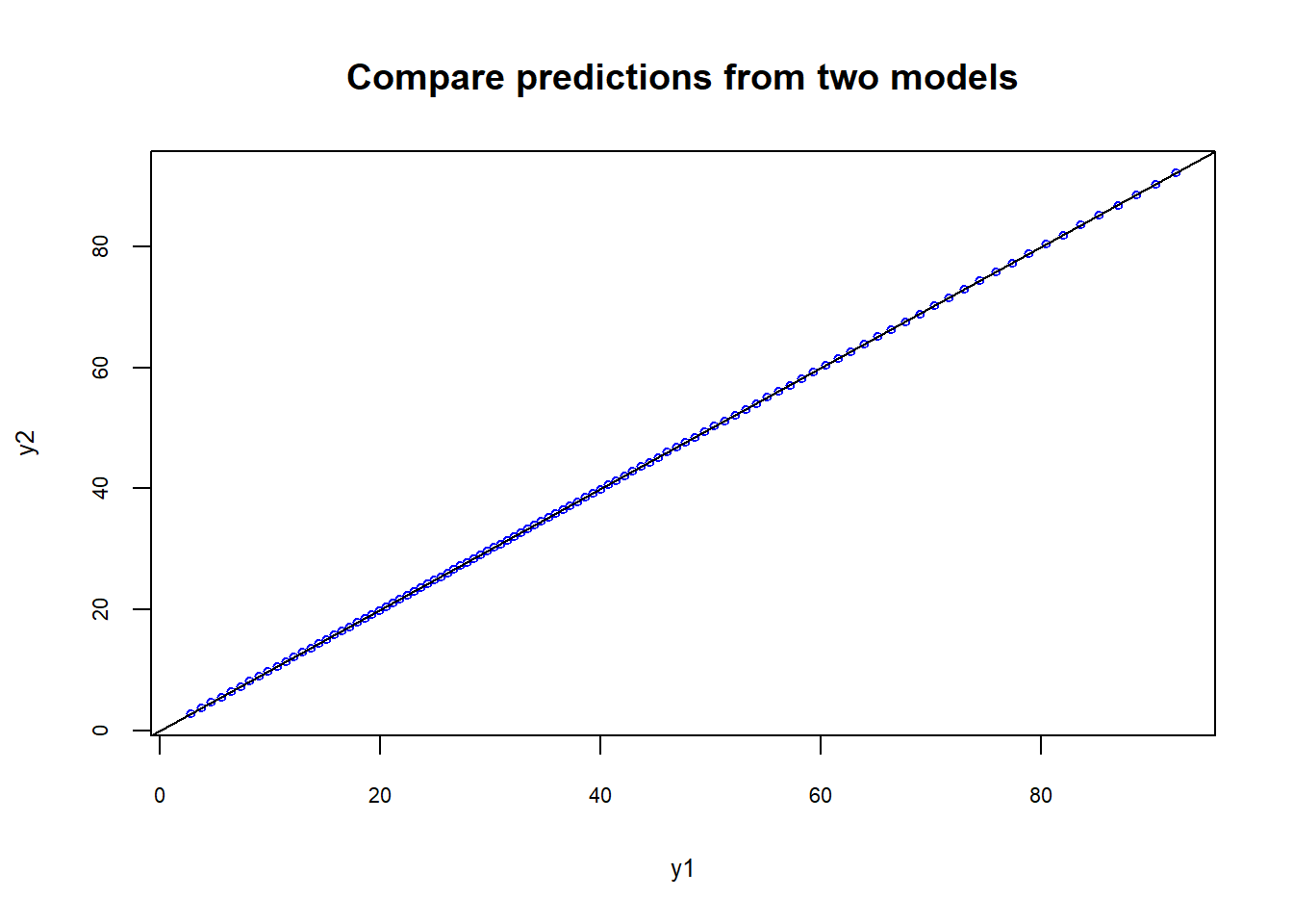
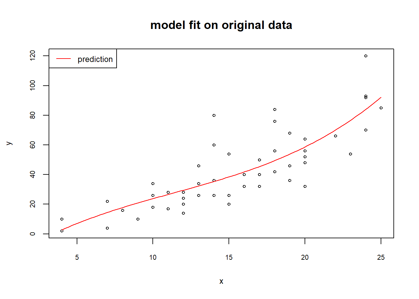
As you see in the plots below, the predictions from the two models are essentially the same and fit the original data very well.

# compare y1 and y2
plot(y1,y2, cex=0.6, col="blue", cex.lab=0.8, cex.axis=0.7, main="Compare predictions from two models")
abline(0,1,col="black")

# also check the fit of the prediction with the original data
plot(x,y, cex=0.6, cex.lab=0.8, cex.axis=0.7, main="model fit on original data")
lines(newx,y1,col="red")
legend("topleft",legend="prediction", lty="solid", col="red", cex=0.8)

Conclusions

1. one can use poly() and lm() to fit polynomial models in R.

2. actually, one can directly specify lm(y ~ poly(x, degree)) to fit models. In this case, the new data should also be given as raw x without any polynomial conversion.

3. raw and orthogonal transformed polynomials make difference only in the term cofficients of models, but have no effect on the predictions.