Introduction
Simpson’s paradox occurs when the direction of an association reverses after data from several groups are combined. For example, A can have a higher success rate than B in every subgroup, yet a lower success rate overall.
In this post, we will simulate exam outcomes in Python, examine the reversal using logistic regression and a plotnine figure, and explain why it happens. All Python code is embedded in this R Markdown document and runs through reticulate.
Setup
You can skip this section unless you want to run the code yourself.
We use NumPy to simulate outcomes, pandas to summarize the data, statsmodels to fit logistic regression models, and plotnine to create the figure. The R package reticulate lets us run Python code within this document. If needed, install it with install.packages("reticulate").
I used the python points to my local executable at /mnt/windows/Program/ubuntu/pyenv/versions/3.13.9/bin/python. To find the python3 executable on your PATH, run:
Sys.which("python3")The setup chunk uses reticulate::use_python() to select a specific Python executable. Replace the path with the executable for your own Python installation or virtual environment before running any Python chunks. If the RETICULATE_PYTHON environment variable is set, it takes precedence over use_python().
Install the Python packages in the same environment. In the command below, replace python with your chosen executable if necessary:
python -m pip install numpy pandas plotnineYou will also need statsmodels for the regression models below. Reticulate runs all Python chunks in a shared session, so objects created in one chunk remain available in subsequent chunks.
A simulated example with a confounding factor
We will examine the relationship between study program and exam pass rate, with exam difficulty as a confounding factor.
Students belong to either program A or program B and choose between an easy exam and a hard exam. We deliberately make their choices uneven: 90% of students in program A choose the hard exam, while 90% of students in program B choose the easy exam.
The table below gives the number of students and the probability of passing for each combination of program and exam difficulty.
| Program | Exam difficulty | Students | Pass probability |
|---|---|---|---|
| A | Easy | 1,000 | 90% |
| A | Hard | 9,000 | 40% |
| B | Easy | 9,000 | 80% |
| B | Hard | 1,000 | 30% |
Using these group sizes and probabilities, let’s simulate a dataset of 20,000 students. Each row represents one student, and the outcome is coded as 1 for a pass or 0 for a failure.
We keep the group sizes fixed and generate each student’s outcome independently with rng.binomial(1, p), where p is the pass probability for that student’s group. A fixed random seed makes the example reproducible.
import numpy as np
import pandas as pd
# Fixed group sizes; independently simulate each student's pass/fail outcome.
rng = np.random.default_rng(2026)
design = [
    ("Easy", "A", 1000, 0.90),
    ("Easy", "B", 9000, 0.80),
    ("Hard", "A", 9000, 0.40),
    ("Hard", "B", 1000, 0.30),
]
df = pd.concat(
    [
        pd.DataFrame({
            "difficulty": difficulty,
            "program": program,
            "passed": rng.binomial(1, probability, size=n),
        })
        for difficulty, program, n, probability in design
    ],
    ignore_index=True,
)
Here are the first few rows of the simulated dataset:
print(df.head()) difficulty program passed
0 Easy A 1
1 Easy A 1
2 Easy A 1
3 Easy A 1
4 Easy A 1We can check the number of students in each group:
df[["program","difficulty"]].value_counts().reset_index(name="Count") program difficulty Count
0 A Hard 9000
1 B Easy 9000
2 A Easy 1000
3 B Hard 1000Examine the pass rates in the simulated data
First, let’s fit a logistic regression model with program as the only predictor of whether a student passes.
import statsmodels.formula.api as smf
logit_fit = smf.logit("passed ~ C(program)", data=df).fit(disp=False)
print(logit_fit.summary())
Logit Regression Results
==============================================================================
Dep. Variable: passed No. Observations: 20000
Model: Logit Df Residuals: 19998
Method: MLE Df Model: 1
Date: Sun, 25 Oct 2026 Pseudo R-squ.: 0.07323
Time: 22:15:47 Log-Likelihood: -12511.
converged: True LL-Null: -13499.
Covariance Type: nonrobust LLR p-value: 0.000
===================================================================================
coef std err z P>|z| [0.025 0.975]
-----------------------------------------------------------------------------------
Intercept -0.2322 0.020 -11.534 0.000 -0.272 -0.193
C(program)[T.B] 1.3197 0.031 43.140 0.000 1.260 1.380
===================================================================================The coefficient for program B, relative to program A, is 1.3197 on the log-odds scale. This positive coefficient indicates that students in program B have a higher probability of passing. The small p-value shows that the association is statistically significant.
Now let’s add exam difficulty to the model:
logit_fit_with_confounder = smf.logit("passed ~ C(program) + C(difficulty)", data=df).fit(disp=False)
print(logit_fit_with_confounder.summary())
Logit Regression Results
==============================================================================
Dep. Variable: passed No. Observations: 20000
Model: Logit Df Residuals: 19997
Method: MLE Df Model: 2
Date: Sun, 25 Oct 2026 Pseudo R-squ.: 0.1441
Time: 22:15:47 Log-Likelihood: -11554.
converged: True LL-Null: -13499.
Covariance Type: nonrobust LLR p-value: 0.000
=========================================================================================
coef std err z P>|z| [0.025 0.975]
-----------------------------------------------------------------------------------------
Intercept 1.8555 0.059 31.210 0.000 1.739 1.972
C(program)[T.B] -0.4760 0.058 -8.185 0.000 -0.590 -0.362
C(difficulty)[T.Hard] -2.2809 0.059 -38.892 0.000 -2.396 -2.166
=========================================================================================After we account for exam difficulty, the coefficient for program B becomes negative. The model now indicates that students in program B have a lower probability of passing than students in program A when exam difficulty is held constant.
To see the reversal directly, let’s compare the pass rates within each difficulty group with the overall rates for each program:
by_group = (
    df.groupby(["difficulty", "program"])["passed"]
    .agg(n="size", passes="sum", rate="mean")
    .reset_index()
)
pooled = (
    df.groupby("program")["passed"]
    .agg(n="size", passes="sum", rate="mean")
    .reset_index()
)
print("Within difficulty groups:")
print(by_group.to_string(index=False, float_format="%.4f"))
print("\nAll students combined:")
print(pooled.to_string(index=False, float_format="%.4f"))
Within difficulty groups:
difficulty program n passes rate
Easy A 1000 886 0.8860
Easy B 9000 7169 0.7966
Hard A 9000 3536 0.3929
Hard B 1000 310 0.3100
All students combined:
program n passes rate
A 10000 4422 0.4422
B 10000 7479 0.7479Plotting these rates side by side makes the reversal easy to see. The first two panels compare programs within each difficulty group; the third combines all students:
from plotnine import (
    aes, facet_wrap, geom_col, geom_text, ggplot, labs,
    scale_fill_manual, scale_y_continuous, theme, theme_minimal,
)

plot_data = pd.concat(
    [by_group, pooled.assign(difficulty="Combined")], ignore_index=True
)
plot_data["difficulty"] = pd.Categorical(
    plot_data["difficulty"], categories=["Easy", "Hard", "Combined"], ordered=True
)
plot_data["label"] = plot_data["rate"].map(lambda rate: f"{rate:.1%}")

plot = (
    ggplot(plot_data, aes(x="program", y="rate", fill="program"))
    + geom_col(width=0.65)
    + geom_text(aes(label="label"), va="bottom", nudge_y=0.02, size=10)
    + facet_wrap("difficulty", nrow=1)
    + scale_fill_manual(values={"A": "#0072B2", "B": "#D55E00"})
    + scale_y_continuous(
        limits=(0, 1), breaks=[0, 0.25, 0.5, 0.75, 1],
        labels=lambda values: [f"{value:.0%}" for value in values],
    )
    + labs(
        title="Simpson's paradox: the comparison reverses when groups are pooled",
        subtitle="Program A has a higher pass rate in each difficulty group",
        x="Program", y="Pass rate",
        caption="Simulated data: A has 90% hard cases; B has 90% easy cases.",
    )
    + theme_minimal(base_size=12)
    + theme(legend_position="none", figure_size=(10, 4))
)
plot.show()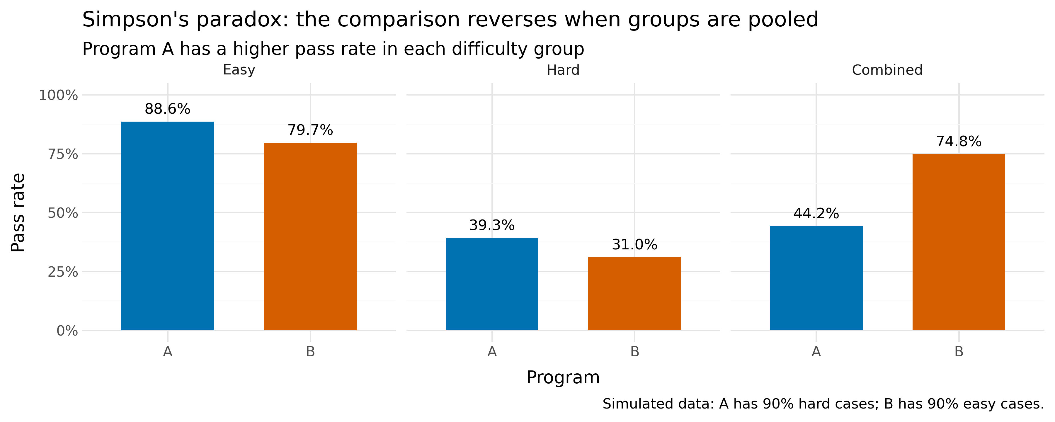
Figure 1: Pass rates within difficulty groups and after pooling students.
Why combining the groups changes the result
Each program’s overall pass rate is a weighted average of its pass rates on easy and hard exams. The weights are the proportions of students taking each exam within that program.
For program A, 10% of students take the easy exam and 90% take the hard exam. Its overall pass rate is therefore:
A: (1,000 / 10,000) × (886 / 1,000)
 + (9,000 / 10,000) × (3,536 / 9,000)
 = 0.4422 = 44.22%
For program B, the proportions are reversed: 90% take the easy exam and 10% take the hard exam. Its overall pass rate is:
B: (9,000 / 10,000) × (7,169 / 9,000)
 + (1,000 / 10,000) × (310 / 1,000)
 = 0.7479 = 74.79%
A has a higher pass rate at each difficulty level, but most of its students take the hard exam. B has a lower pass rate at each difficulty level, but most of its students take the easy exam. Because the subgroup rates receive different weights, the overall comparison favors B.
The reversal is already present in the probabilities we specified, before we simulate any outcomes. Using those probabilities, the expected overall pass rates are:
A: 0.10 × 0.90 + 0.90 × 0.40 = 0.45
B: 0.90 × 0.80 + 0.10 × 0.30 = 0.75
Random sampling introduces variation around these expected rates. The reversal itself comes from the combination of pass probabilities and the uneven distribution of exam difficulty across programs.
Difficulty is a confounder here
In this simulation, students in program A are more likely to choose hard exams than students in program B. Exam difficulty is therefore associated with program membership, and it also affects the probability of passing. It plays the role of a confounder: ignoring it mixes the association between program and passing with differences in exam difficulty. Accounting for difficulty lets us compare the programs among students taking exams of the same difficulty.
A reversal alone does not establish a causal effect or tell us which variables to adjust for. Those decisions require assumptions about how the variables relate. For example, conditioning on a collider can introduce bias. Dividing the data into subgroups based on every available variable is therefore not a general solution.
Takeaways
- Simpson’s paradox occurs when an association points in the same direction within every subgroup but reverses when the groups are combined.
- Examine group sizes as well as rates: differences in group composition determine the weights in the overall comparison.
- Use knowledge of the data-generating process to guide causal interpretation and adjustment.
Last modified on 2026-10-23