Example 1: Basic Usage of legend.position

The simplest way to move a legend inside the plot is by providing a numeric vector of length two to the legend.position argument in theme(). These coordinates represent the relative position within the plot panel, ranging from 0 to 1. Check the section on “Key Positioning Controls” at the end for a detailed explanation of the coordinate system.

library(ggplot2)

ggplot(mtcars, aes(wt, mpg, color = factor(cyl))) +
  geom_point(size = 3) +
  theme_bw() +
  theme(legend.position = c(0.8, 0.8))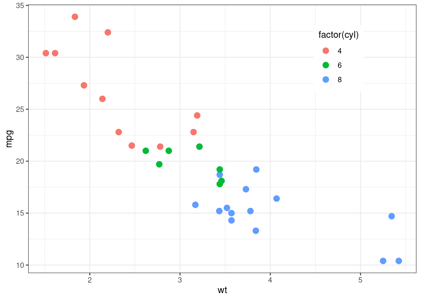

Example 2: Fine-Tuning with Justification and Background

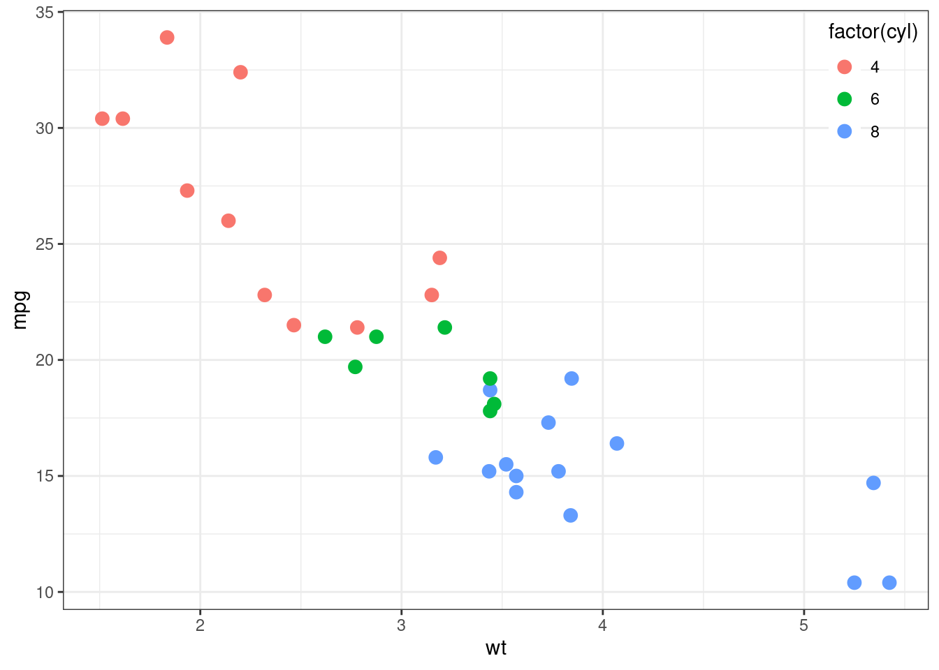
When you place a legend inside, you often need to adjust which part of the legend box aligns with your coordinates and handle the background if it obscures data.

• legend.justification: Controls the anchor point of the legend box. For example, c("right", "top") means the top-right corner of the legend box will be placed at the specified coordinates.
• legend.background: Use element_blank() to make the background transparent.

ggplot(mtcars, aes(wt, mpg, color = factor(cyl))) +
  geom_point(size = 3) +
  theme_bw() +
  theme(
    legend.position = c(1, 1),
    legend.justification = c("right", "top"),
    legend.background = element_blank()
  )

Example 3: Positioning in Faceted Plots

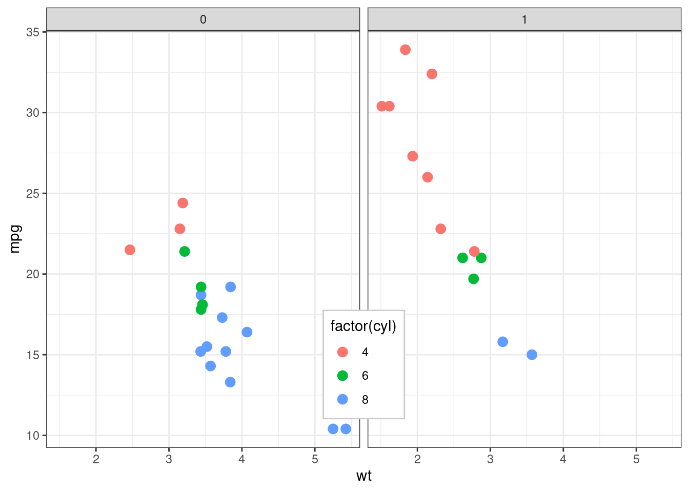
Moving the legend inside a faceted plot works similarly: the whole figure is considered as one plot for the coordinate system. You can use the coordinates to place it within one of the empty spaces or over a specific panel. In the following example, the legend is placed in the bottom center of the plot, and a background is added to improve readability:

ggplot(mtcars, aes(wt, mpg, color = factor(cyl))) +
  geom_point(size = 3) +
  facet_wrap(~am) +
  theme_bw() +
  theme(
    legend.position = c(0.5, 0.2),
    legend.background = element_rect(fill = "white", color = "grey80")
  )

Example 4: The “Empty Space” Trick for Faceted Plots

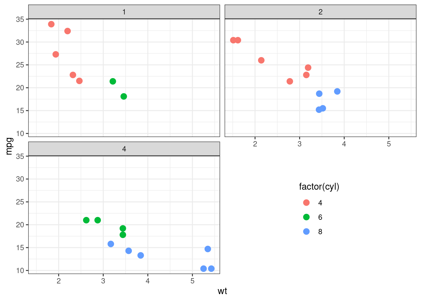
If you have a panel which doesn’t have any data, and then it is the perfect spot to place legend. To show this, the facet variable carb has only 3 values, and we will make a 2x2 facet grid. We will also remove the background and border of the legend. The following example shows this:

# Use 3 categories to leave the 4th spot in a 2x2 grid empty
mtcars_subset <- mtcars[mtcars$carb %in% c(1, 2, 4), ]

ggplot(mtcars_subset, aes(wt, mpg, color = factor(cyl))) +
  geom_point(size = 3) +
  facet_wrap(~carb, nrow = 2, ncol = 2) +
  theme_bw() +
  theme(
    # Coordinates c(0.75, 0.25) target the center of the empty bottom-right area
    legend.position = c(0.75, 0.25),
    legend.background = element_blank(),
    legend.justification = "center"
  )

Key Positioning Controls

To master legend positioning, keep these three controls in mind:

1. Coordinate System: The coordinates c(X, Y) represent a relative scale from 0 to 1 across the plot panel.
   • c(0, 0): Bottom-left corner
   • c(1, 1): Top-right corner
   • c(0.5, 0.5): Center of the plot
2. Anchor Point (legend.justification): Use this to control which part of the legend box aligns with your coordinates. For example, c("right", "top") ensures the top-right corner of the legend box sits exactly at your target coordinate.
3. Background Removal: If your legend blocks data points, clear the legend box background using legend.background = element_blank(). Alternatively, use element_rect() to give it a semi-transparent or styled background.

Happy Programming!